Bayesian Network Representation of Joint Normal Distributions - Confounding Variables Model

This post is the second of a series discussing the Bayesian Network representation of multivariate normal distributions. In the first post we introduced a cascading regressions model leading to a Bayesian network representation of any joint normal distribution [DP22]. A joint normal distribution being fully specified by its mean vector and its covariance matrix is not simple to interact with as its Bayesian network equivalent. Representing a joint normal distribution as a Bayesian network enables visualizing and interact the distribution through the lens of probabilistic graphical models with TKRISK®.

We demonstrate in this post a simple yet powerful approach using a confounding variables model.

A normal distribution $\mathcal{N}(m, v)$ is fully specified using two parameters: its mean $m\in\mathbb R$ and its variance $v\in\mathbb R_+$. Likewise, a $n$-dimensional multivariate normal distribution $\mathcal{N}(M, V)$ is fully specified by its mean vector $M\in\mathbb R^n$ and covariance matrix $V\in\mathbb R^n\times\mathbb R^n$.

The latter can also be represented as a Bayesian Network, more specifically as a Gaussian Bayesian network [KF09] [IC20].

In what follows we will be working with a vector of random variables $X=(X_1,..., X_n)$ following a multivariate normal distribution $\mathcal{N}(M, V)$.

By definition $M = (\mathbb E[X_i])_{i \in \llbracket 1, n\rrbracket}$ and $V = (cov(X_i, X_j))_{(i,j) \in \llbracket 1, n\rrbracket^2}$.

Through basic matrix operations we will show how $\mathcal{N}(M, V)$ can be represented through a confounding variables model which is a particular case of a linear Gaussian Structural Equation Model (SEM) [MD11] [GP19], the latter having a direct Gaussian Bayesian Network equivalent.

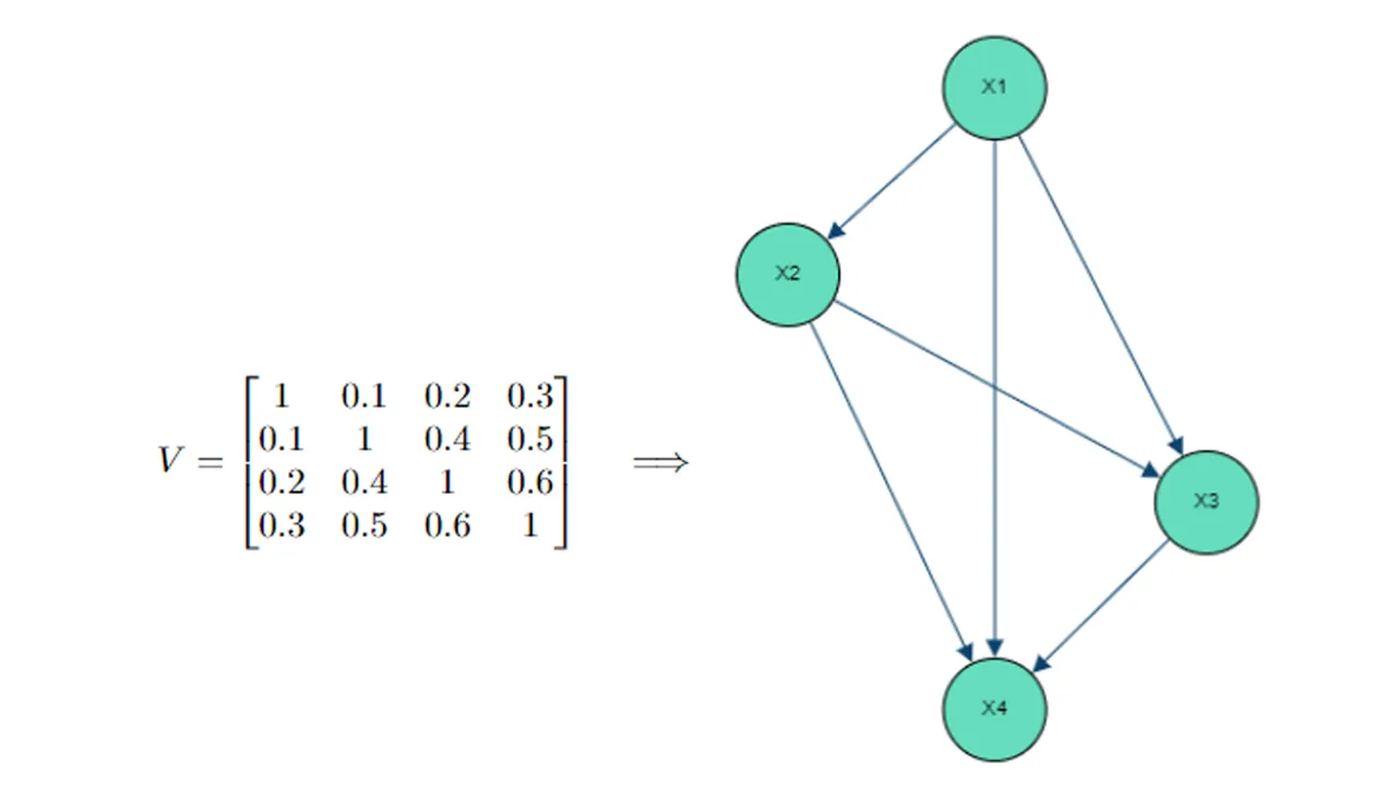
Applying LDL decomposition on $V$ yields $V = L D L^T$ with $L$ being unit lower triangular and $D$ diagonal.

Therefore:$$X - M\sim L E$$ with $E\sim \mathcal{N}(0, D)$.

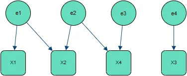
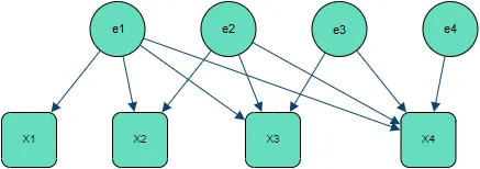
Instead of rewriting equation as in [DP22] leading to the cascading regressions model, we can directly interpret $E$ as a set of confounding variables. In writing the regression model as:$$X_i = m_i + \sum_{j=1}^{i-1}l_{ij}e_j + e_i$$with $L=(l_{ij})_{1\leq i,j \leq n}$, we obtain a direct Gaussian Bayesian Network representation where the variables $(e_i)_{1\leq i \leq n}$ are confounding, meaning these are not observed, however allow introducing a correlation structure among observed ones ($X_1, ..., X_n$ in our case).

In this case $Pa(X_i) = \{e_1, ..., e_{i-1}\}$.

It is important to note that a different order in the variables will lead to a different Bayesian Network structure, representing however the exact same joint distribution.

Like for the cascading regressions model [DP22], the above approach is simple, computationally efficient and allows Bayesian Networks generation straight from any dataset for which variables are assumed normally distributed.

The LDL decomposition is here sufficient to obtain all Bayesian network parameters and allows handling any case of covariance matrix (even non definite) and thus any multivariate normal distribution. The simplicity of the algorithm comes at the cost of additional variables - the confounding variables.

It is common to work on standardized normal distributions, i.e. with zero mean and unit variance:

• $M=0$
• $\textit{Diag}(V) = [1, \cdots, 1]$

In this case covariance and correlation matrices are one and the same. This is a convenient setup which does not imply loss of generality as non-normalized marginals can be recovered by shifting and scaling the normalized ones. Working on normalized space allows for direct comparison of dependencies between variables as these are independent of their actual magnitude.

For a self-contained graph representation, contrary to the above generic approach, the Gaussian Bayesian Network is insufficient and would require additional deterministic nodes to apply shifting and scaling (shifting and scaling directly a node on the Bayesian Network would propagate on its children and thus alter the joint distribution).

For sake of simplicity we will present examples on standardized normal distributions only.

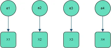
To visualize and interpret the above approach, we will take basic examples of 4 dimensional multivariate normal distributions.

$V = \begin{bmatrix}1 & 0 & 0 & 0 \\0 & 1 & 0 & 0 \\0 & 0 & 1 & 0\\0 & 0 & 0 & 1\\\end{bmatrix}$ $\implies$

$V = \begin{bmatrix}1 & 0.1 & 0 & 0 \\0.1 & 1 & 0 & 0.5 \\0 & 0 & 1 & 0\\0 & 0.5 & 0 & 1\\\end{bmatrix}$ $\implies$

$V = \begin{bmatrix}1 & 0.1 & 0.2 & 0.3 \\0.1 & 1 & 0.4 & 0.5 \\0.2 & 0.4 & 1 & 0.6\\0.3 & 0.5 & 0.6 & 1\\\end{bmatrix}$ $\implies$