How water is the Main Driver of Oilfields Greenhouse Gases Emissions
This post overturns the conventional belief that greenhouse gas (GHG) emissions from oil fields peak at the beginning of their operational life. Analyzing a conventional oil field over 40 years, we find that GHG emissions and carbon intensity (CI) instead show significant variability and an increase as the field matures, particularly due to increased water production that requires more energy-intensive extraction processes. These findings challenge existing emission models and underscore the need for strategic operational adjustments, such as Enhanced Oil Recovery (EOR) and optimized water management, to mitigate late-life emissions. The Oilfield Pollutant Graphical Model (OPGM) calls for a reevaluation of life-cycle emission assessments and emphasizes the importance of adopting new technologies and practices for sustainable hydrocarbon production.
Oil fields produce large volumes of fluids (on the order of ). Although direct emissions of greenhouse gases (GHGs) (carbon dioxide, methane, etc.) are often referred to as the main contributors, other operations in the field can result in emissions that display higher variability and sensitivity to external factors. Another misconception is that the emissions and CI are higher early in the life of the field, as the construction of facilities (pipelines, wells, gathering centers) leads to more fugitives. The Oilfield Pollutant Graphical Model (OPGM) ([5]) allows us to accurately quantify the emissions of each process in the upstream and midstream supply chain of a field and to measure the impact of changes in operating conditions on overall emissions. In this work, we show how, tracking the evolution of emissions and CI through the life of the field, daily emissions vary widely and tend to increase toward the end of life. We conducted a comprehensive evaluation of a large conventional oilfield over 40 years and showed the profile of Field Emissions (FE) and Carbon Intensity (CI) over that period.
We present an analysis of the emissions of a waterflooding oil field over its useful life (approximately 45 years). This highlights how different phases of operations lead to varying emissions patterns and CI. Until then, most of the analyzes using OPGEE ([4]) focused on average emissions using a single-time-step approach.
OPGM allows us to seamlessly perform time-dependent estimations. To illustrate, we use a synthetic field whose characteristics are presented in Table [1].
| Property | Value |
|---|---|
| Location | Offshore |
| Fluid | Oil |
| Reserves | 450 MMB |
| Reservoir Depth | 3400 ft |
| Reservoir Temperature | 131 F |
| API | 18 |
| Number of Producers | 5 |
| Number of Injectors (W/G) | 3/2 |
| Plateau | 70 MBPD |
| GOR | 1250 stb/scf |
| FOR | 100-900 |
| Venting fraction | 0.002 |
| Flaring combution efficiency | 93.2% |
| Water injection rate/well | 15 MBPD |
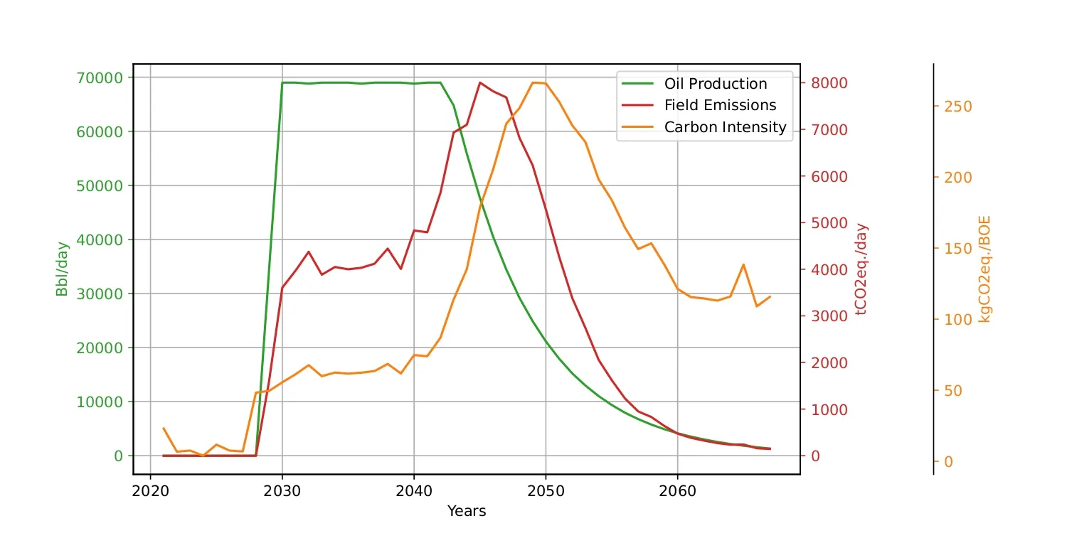
The field production profile is presented in Figure [1]
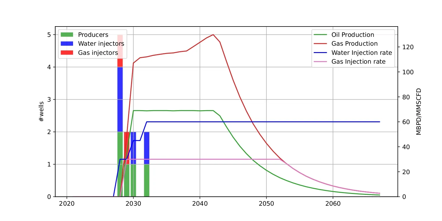
This profile shows a plateau production that lasts 13 years. Note the increase in gas production during the plateau years as a result of the depressurization of the reservoir. We also assume that water production increases over time. The reservoir model hypothesis is presented in the appendix.
Both the water and the gas produced are re-injected into the reservoir for disposal and as a pressure maintenance strategy, keeping a Voidage Replacement Ratio (VRR) between 50% and 75% for most of the recovery period. This model accounts for the gas separation within the reservoir under the effect of depletion.
The flaring-to-oil ratio (FOR) is a constant fraction of the gas-oil ratio (GOR).
For every year of operations, we run OPGM taking as input the field's data (fluid volumes, pressure, ratios) and generating the field's emissions (tCO2eq/d) and CI (kgCO2eq/BOE). Figure [2] shows how the emission profile evolves with production.
We note that the field's emissions increases towards the end of the plateau life. To understand where this uptick comes from, we can breakdown the field's total emissions into seven categories.
Downhole pump
Separation
Flaring
Venting
Water injection
Vapor Recovery Unit (VRU)
Upstream
Figure [3] shows the evolution of each category, in absolute and relative to the total field's emissions:
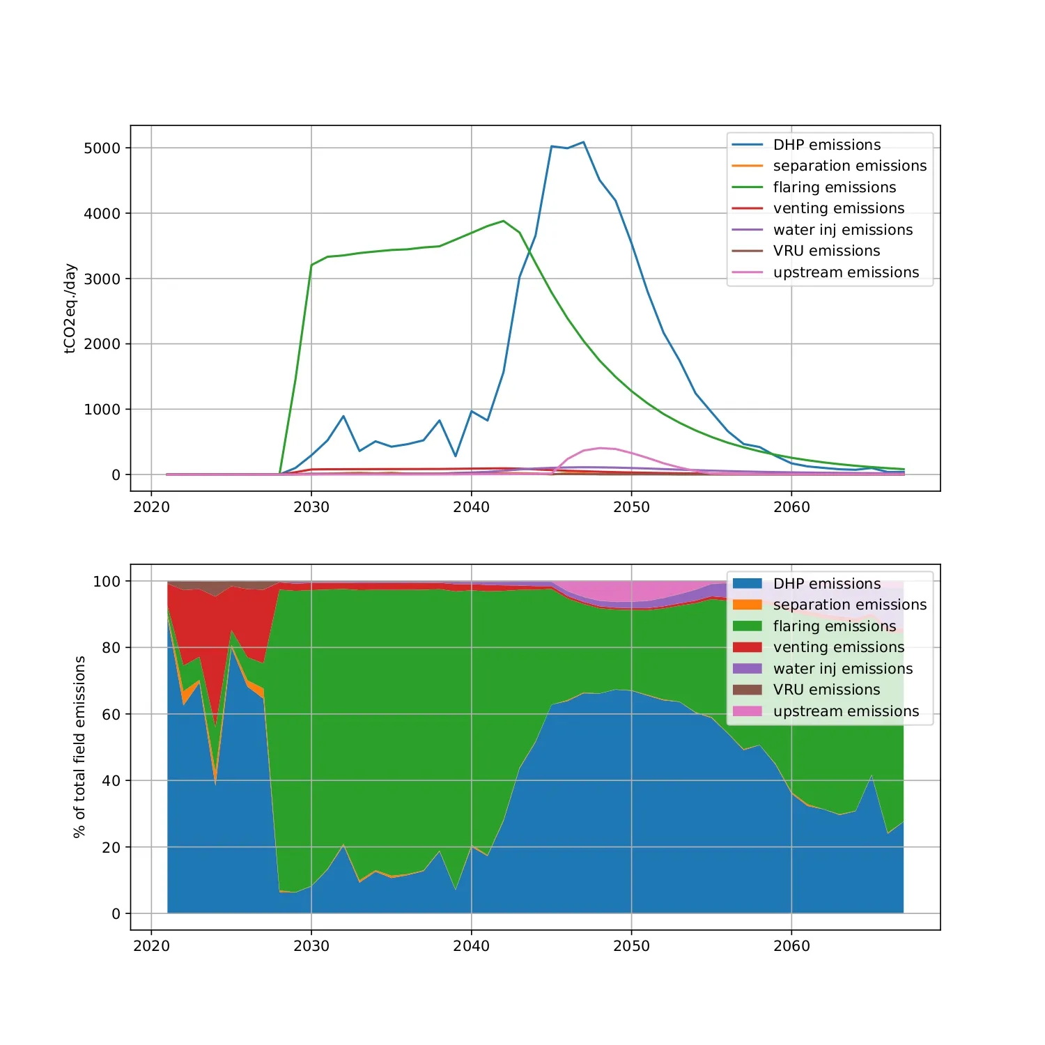
We note that while flaring is the main contributor while gas production remains high, the down-hole pump emissions become overwhelming as the water production increases and the field needs an increasing amount of energy to lift the heavy fluid column out of the reservoir. OPGM offers the possibility of showing an even more granular breakdown, as each node in the graphical model can be "exposed" to the user. This helps diagnose the main contributors to emissions and act appropriately to alleviate them.
Artificial lift systems are ubiquitous in oil and gas production. They facilitate the movement of fluids from underground reservoirs to the surface. These systems contribute significantly to greenhouse gas (GHG) emissions, primarily through fugitive emissions and the energy consumed in pumping. Our model includes a down-hole pump module designed to calculate the energy use and associated emissions from artificial lift operations. This module comprises five key components: well-bore conditions, bottom-hole fluid properties, well-bore fluid properties, mass rate, and energy usage and emissions. In particular, energy usage and emissions, along with the mass rate component, are integral to all modules of the system.
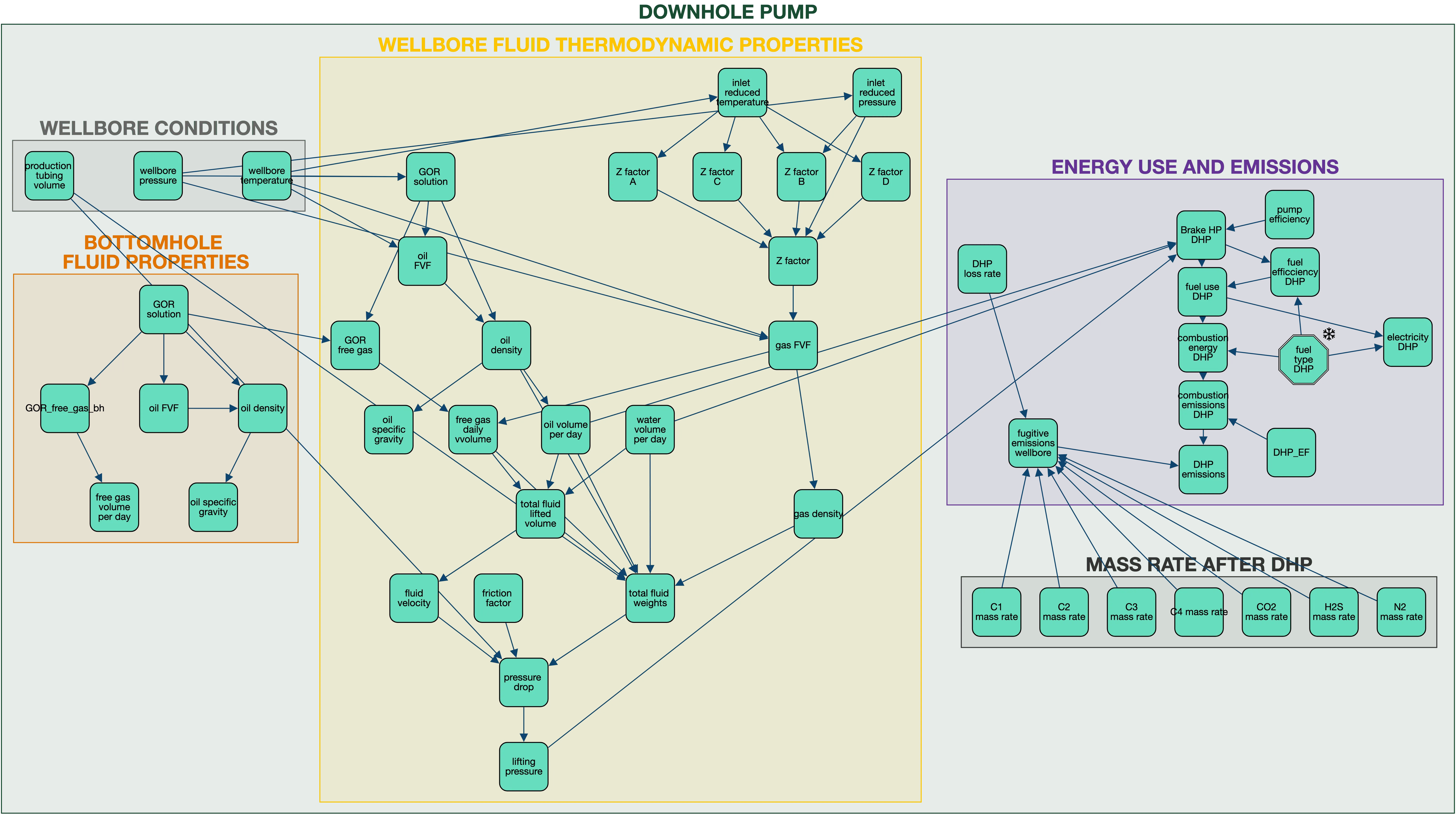
The module includes the following calculations:
Pressure and Energy Calculations: The energy required to lift fluids is calculated based on overcoming the pressure traverse, which includes resistance to gravity flow and frictional losses. The pressure required is the sum of the well head pressure, the pressure traverse, and subtracting wellbore pressure.
Fluids and Properties: This part involves calculating the average properties of the fluids within the wellbore, such as pressure, temperature, and density. These calculations take into account variables like the gas-oil ratio, as well as wellhead and wellbore conditions.
Well Pressure Traverse: This involves calculating the gravitational head, which is the pressure drop due to gravity, and the frictional pressure drop resulting from fluid contact with the well tubing. The calculation uses fluid density, wellbore volume, and tubing cross-sectional area.
Pump Power and Efficiency: The brake horsepower of a pump is calculated using its discharge flow rate, pumping pressure, and efficiency. The pumping pressure differs between the pump discharge and the suction pressures.
The Security and Exchange Commission (SEC) rule on oil and gas reserves [6] stipulates that booked reserves must be produced economically. International oil companies are sometimes constrained to write down a large portion of their assets as a result of oil price changes or increased operating costs. As an example, Royal Dutch Shell had to take a 22 Billions dollars in write down in June 2020 after demand dropped following the outbreak of the COVID pandemic. A field will continue to produce its wells as long as they are economic (that is, they bring more revenue than what it takes to operate them). This economic limit is typically computed when the operating gross income (gross revenue - royalties - capex - opex) of a field becomes negative. Operating expenditure consists of a fixed and variable part, which depends on the volumes produced. If producing less water means a lower OPEX, in general, this becomes even more important when we consider the associated GHG and the costs they could incur. A preliminary analysis indicates that this may reduce the life of a field by more than 10 years. This would have a major impact on the reserves valuation of an asset (and, therefore, the companies that own it).
This study dismantles the prevalent assumption that GHG emissions from oil fields are highest at the start of production. Through the deployment of OPGM, our analysis over the 40-year lifespan of a conventional oil field reveals a more complex reality: emissions do not peak early but instead exhibit significant variability, with a notable increase as the field matures. This trend is mainly attributed to the increased production of water along with oil, necessitating greater energy for extraction and, consequently, higher emissions.
This counterintuitive finding highlights the need for strategic operational adjustments. As fields age, adopting practices that favor a more efficient fluid displacement, such as enhanced oil recovery (EOR), and optimizing water handling, can mitigate emissions. Moreover, they would result in improvements in KPIs that affect the returns and valuation of incumbent companies.
In conclusion, this insight calls for a reevaluation of life-cycle emission models in policy formulation and the industry's approach to managing aging fields. While data-driven approaches tend to model the future as an extension of the present, foresight leading to actionable items will come from expert driven models such as OPGM.
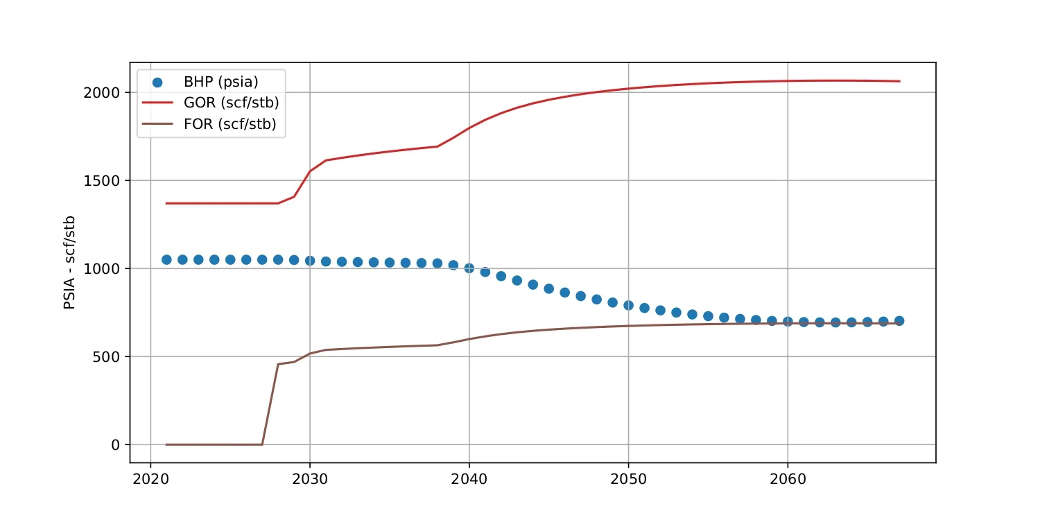
The reservoir model we employ is based on the principle of material balance, which ensures the conservation of mass within the reservoir. This principle illustrates how fluid extraction affects reservoir pressure and fluid dynamics. As fluids are withdrawn, the resultant void causes a pressure drop, leading to expulsion of gases previously dissolved in liquid phases. This phenomenon results in an increase in the field's overall gas production. We postulate that a constant fraction of the gas production is lost in fugitive emissions. These can be significant contributors to carbon intensity (CI) since methane is a gas with a much higher GHG potential than . Figure [5] shows the joint evolution of the GOR, FOR and bottom hole pressure.
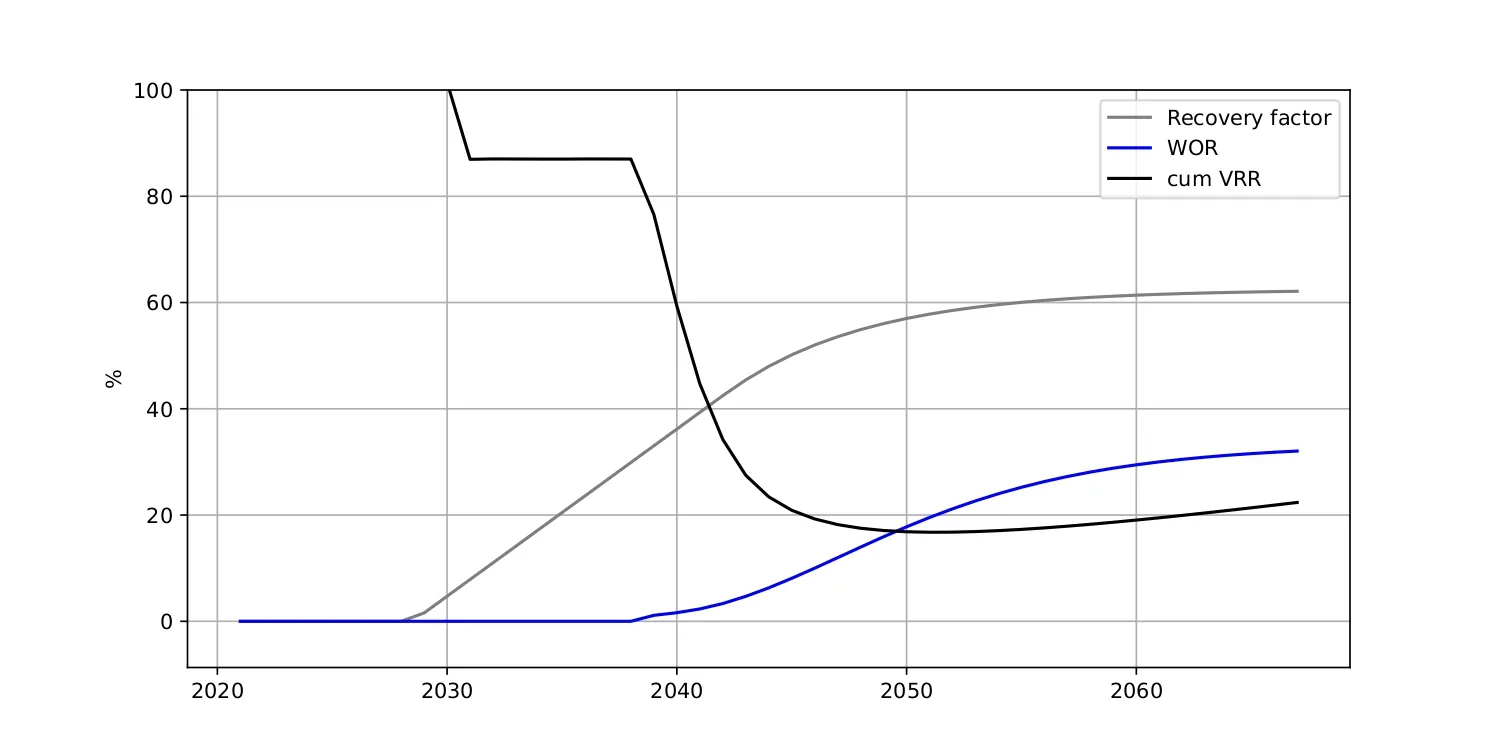
To counteract pressure depletion, voidage replacement strategies, such as water or gas injection, are employed, stabilizing pressure, and sustaining production. Similarly, as fluids are extracted from the reservoir, formation, and injected water take their place, and we typically see an increase in water production. We use a water oil ratio (WOR) vs. recovery type curve to model this behavior. [6] shows how these ratios evolve with time.
The energy consumption calculated from each process must be converted into fuel use by looking up the fuel use factor of the primary mover. OPGEE provides four types of drivers for pumps, compressors, and onsite electricity generators. Drivers include natural gas-powered engines, gas turbines, diesel engines, and electric motors. Table [2] shows the types and size ranges of the drivers included in the model.
| Type | Fuel | Size range [bhp] | Reference |
|---|---|---|---|
| Internal combustion engine | Natural gas | 95 - 2,744 | [1] |
| Internal combustion engine | Diesel | 1590 - 20,500 | [1] |
| Simple turbine | Natural gas | 384 - 2,792 | [2] |
| Motor | Electricity | 1.47 - 804 | [3] |
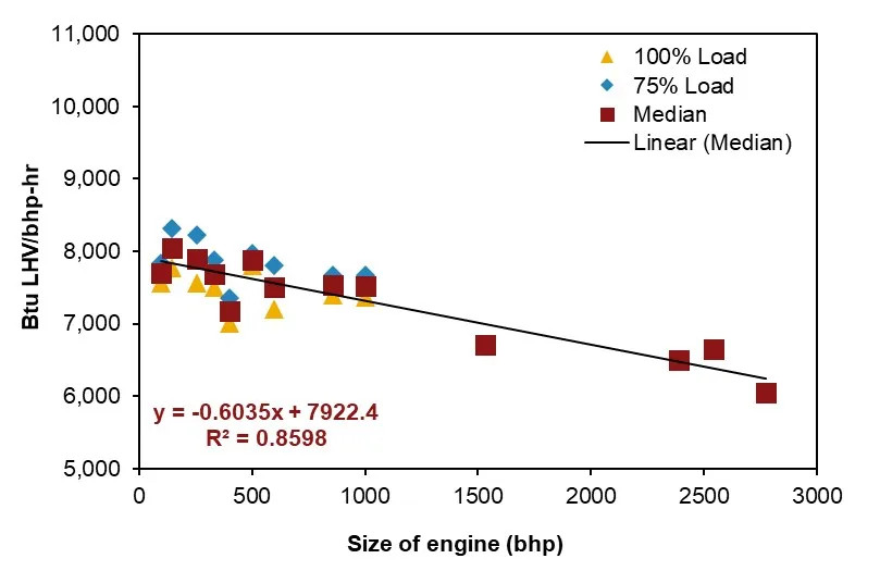
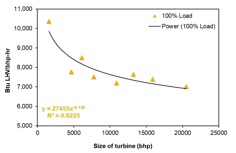
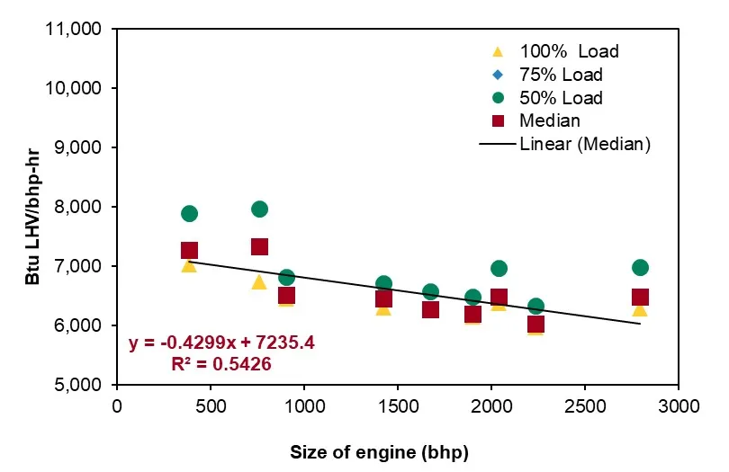
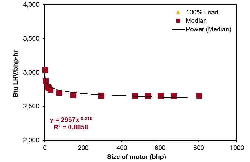
In the process, the primary mover type is chosen from either the default of the user or the model. Given the type of primary mover and the horsepower of the brake, the efficiency of the primary mover is calculated using the correlations in Figure [7]. The figure collects data from the reference in Table [2], including the size, efficiency, and power load of the engine from the various types of real-world drivers to generate the correlation. The correlation between engine size and efficiency is generated using the median load for natural gas engines, diesel engines, and electric motors and 100% load for natural gas turbines (the data we collected is 100% load). The correlation expressions are in the left-hand corner of each sub-figure in Figure [7]. The R-squares of the correlations are 0.86, 0.82, 0.54, and 0.85, respectively. Fuel consumption of the selected primary mover type can be calculated in each process using these expressions.
In particular, the model assumes the 100% use of the natural gas produced for the combustion of natural gas on site. Table [3] lists the combustion technologies and fuels included in the model:
| Natural gas | Diesel | Crude | Residual oil | Pet. coke | Coal | |
|---|---|---|---|---|---|---|
| Industrial boiler | ✓ | ✓ | ✓ | ✓ | ✓ | ✓ |
| Turbine | ✓ | ✓ | ||||
| CC gas turbine | ✓ | |||||
| Reciprocating engine | ✓ | ✓ |